Hello, World!

LED blinking is the de-facto Hello, World! example for Embedded System. You got to stay true to that tradition, hence our example will use an LED. But instead of blinking, we will fade in - fade out the LED. Now, if you are familiar with Embedded System you know you can do that using PWM. But, instead, we will apply a Sinusoidal analog signal on the LED.

This will result in LED fading in and out. The sine wave will be generated by a Neural Network model.

Note: This example might sound ridiculous, but the goal of the tutorial is to show you how to run a model on a microcontroller. Just like when you started to learn embedded system you started with LED blinking, even when it looked like it wasn’t useful (but it was useful, wasn’t it?). This simple example will allow us to build a simple neural network that is also small enough to run on microcontrollers. Once you get familiar with the basic principles we will explore more challenging examples e.g. speech recognition, image processing, etc.

The development board that I will be using has an LCD, we can plot the sine wave on there too. In a nutshell, I will show you:

• How to build and train a model using TensorFlow
• Convert the model to TFLite Micro with optimizations enabled for hardware
• Convert the model into a C source file that can be included in the microcontroller application
• Run on-device inference and display output

Build and Train a model

Well, what does train a model even mean? It means, we are going to show “the model” some input data and its corresponding output data and will ask it to figure out the relationship between input and output (known as supervised learning). Just like how you teach a toddler, for example, who never saw a dog before. If you show a toddler enough pictures of dogs, she will learn from it and next time when she sees a dog she will be able to ‘guess’ its a dog.

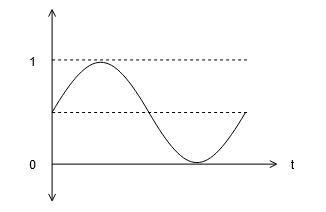
For our example, though, we want to build a sine wave function:

We want a model that can take a value, x, and predicts its sine, y. And to do that we will show the model thousands of samples (x and its corresponding y). The model will learn from it and will be able to predict y for new/unseen x values (this type of problem is called regression).

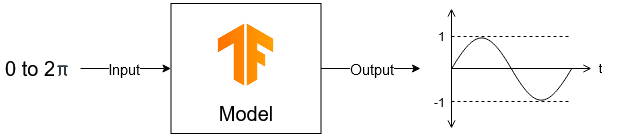
The model will take any value between 0 to 2pi and will predict the output between -1 to 1, without knowing what sine wave is.

For training, we will use Google Colab. It is an online environment to run Python with all the required packages already installed for ML. All you need is a Gmail account. But if you already have everything installed on your workstation, feel free to use so.

The full code can be found here (will open on Google Colab). I will explain the code here. Some of the explanations are written in the google colab too. It will probably be a good idea for you to keep the colab tab and this tab open side by side.

Let’s get started:

• Head over to the Google Colab.
• In Google Colab there are two types of sections. The Code section and the Text section. Text sections are just that, text, to explain the following code and provide you information. Code sections are the ones that you will have to run.
• This is a code section:

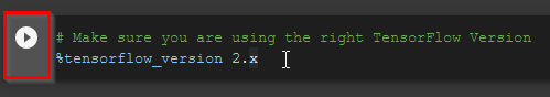
• To run a code section you will have to press the play button. The play button appears when you click anywhere on a code section. When you press play, colab will only execute that part of the code and will print output if there are any.

Generate data

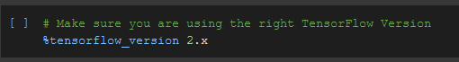
1
%tensorflow_version 2.x

First, we are making sure that we are using the latest TensorFlow (at the time of writing the latest version is 2.1, but you can only choose major versions, 1 or 2).

1
2
3
4
5
import numpy as np
import tensorflow as tf
from tensorflow import keras
import matplotlib.pyplot as plt
import math

Importing all the necessary modules. Keras is the high-level API for the TensorFlow deep learning.

1
SAMPLES = 1500

In the real world, if you want to build a model, for example, for your accelerometer to detect a gesture you will have to collect thousands (if not more) of sample data for that particular gesture to train your model with. But in our case, we know what an ‘ideal’ sine wave looks like. We can simply use Python’s ‘math’ module’s sine function to generate the y values. As we are generating our samples we can decide how many samples we want.

Let’s start with 1500 samples. We will generate uniform random data for x ranging from 0 to 2pi. Also, plot x values to see if they are random or not.

1
2
3
4
x_values = np.random.uniform(low=0, high=2*math.pi, size=SAMPLES)

plt.plot(x_values)
plt.show()

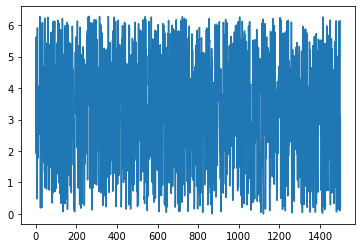
Looks pretty random. If you want to you can shuffle more. Now, let’s generate corresponding y values and plot Y vs X.

1
2
3
4
5
6
np.random.shuffle(x_values)

y_values = np.sin(x_values)

plt.plot(x_values, y_values, 'b.')
plt.show()

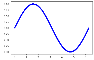
Real-world sensor data are rarely this smooth. They are always noisy, and that’s why we needed a Machine Learning algorithm in the first place. Deep Learning algorithms are best for noisy sensor output and generalize well. So, to reflect real-world situations let’s add some noise to our y values and plot again.

1
2
3
4
y_values += 0.1 * np.random.randn(*y_values.shape)

plt.plot(x_values, y_values, 'b.')
plt.show()

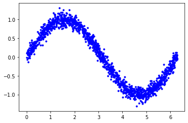
Now the output looks like a noisy output of a sensor.

Once you have data to train your model, it is a standard practice to split the data into several sections, namely, Train, Validation, and Test.

Train data is used during model training. But how would model know how is it doing? That is where Validation data is useful. It will tune its own parameter to generate a model and then check against validation data, data that the model hasn’t seen during training. So, the model itself is checking its own accuracy using unseen (validation) data.

Note: You might come across a situation where you will see that the training results are better than validation results. In that case, it means the model memorizes the training data too well (known as overfitting) and didn’t generalize the relationship between input and output well (we will discuss this more later).

You will mostly go back and forth to tune the algorithm’s parameter until the validation is the same or better than the training metrics. Once you are satisfied, finally you test it using Test data, just to make sure that during the back and forth you didn’t accidentally overfit the validation data too.

The common practice is to use 60% for Training, 20% for Validation, and 20% for Test.

1
2
3
4
5
6
TRAIN_SPLIT = int(0.6 * SAMPLES)
TEST_SPLIT = int(0.2 * SAMPLES + TRAIN_SPLIT)
x_train, x_test, x_validate = np.split(x_values,  [TRAIN_SPLIT, TEST_SPLIT])
y_train, y_test, y_validate = np.split(y_values,  [TRAIN_SPLIT, TEST_SPLIT])

assert  (x_train.size + x_validate.size + x_test.size) == SAMPLES

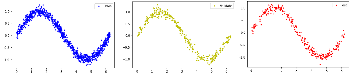
Now, let’s print the split data to see that each of these datasets cover the full range of input (0 to 2pi) and isn’t aggregated on one side.

1
2
3
4
5
6
7
8
9
10
plt.plot(x_train, y_train, 'b.', label="Train")
plt.legend()
plt.show()

plt.plot(x_validate, y_validate, 'y.', label="Validate")
plt.legend()
plt.show()

plt.plot(x_test, y_test, 'r.', label="Test")
plt.legend()

Design the model

In neural network you have neurons (think of it as a node in a mesh network). Each of these neurons has weight and bias values. During training, these values are changed, by an activation function, that you will select during training, to match its prediction with the actual output. A loss function will be used to see how far the predictions are from the actual value and the training process will try to minimize this value.

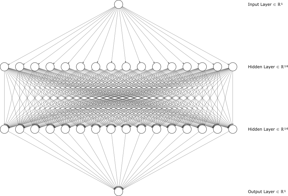
You can have any number of layers of neurons. But, a greater number of neurons leads to more complexity, and hence will also increase the size of the model. We will be using two layers of 16 neurons (i.e. 32 neurons), with one input layer and one output layer. Remember, our input is just one value, x and output is just one value, y. This is what our neural network will look like:

1
2
3
4
5
model = tf.keras.Sequential()
model.add(keras.layers.Dense(16, activation='relu', input_shape=(1,)))
model.add(keras.layers.Dense(16, activation='relu'))
model.add(keras.layers.Dense(1)) # Output Layer
model.compile(optimizer='adam', loss='mse', metrics=['mae'])

We will be using the Sequential model. It is a simple model architecture with layers in series. input_shape refers to input size, which in our case is one. As activation function we used Rectified Linear Unit (ReLU), Adam is the actual algorithm, Mean Squared Error (mse) is our loss function, and to judge our model’s performance we used Mean Absolute Error (mae) metrics.

Note: Details about each of the bold words are outside of the scope of this tutorial. Keras and TensorFlow have a lot of details about each of the choices and their alternatives.

Train the model

During training, the model will predict the output of a corresponding input x and will check how far it is from the actual value. then it will adjust the neurons’ weights and biases to match the actual output.

1
training_info = model.fit(x_train, y_train, epochs=350, batch_size=64, validation_data=(x_validate, y_validate))

Epoch: Training runs this process (adjusting neurons’ weights and biases) on the full dataset multiple times, and each full run-through is known as an epoch. Don’t use a high number of epochs though. Otherwise, the model will overfit their training data.

Batch Size: During each epoch, you can adjust the weights and biases after each input. Or you can update those values in batches. For example, you can use 16 samples, aggregate their correctness results, and then update weights and biases based on that. Choosing 1 as batch size will take forever to train, choosing the whole data as batch size will result in a less accurate model. It is a trial and error situation. The thumb of rule is to start with a batch size of 16 or 32 and increase from there to see what works best for you.

Click play to train the model. It might take a min or two to complete. During each epoch, the model prints out its loss and mean absolute error for training and validation as you can see in the output (note that your exact numbers may differ):

Epoch 350/350
15/15 [==============================] - 0s 4ms/sample - loss: 0.0105 - mae: 0.0809 - val_loss: 0.0108 - val_mae: 0.0803

Let’s plot the loss function output over time for both Training and Validation.

1
2
3
4
5
6
7
8
9
10
11
loss = training_info.history['loss']
validation_loss = training_info.history['val_loss']
epochs = range(1,  len(loss) + 1)

plt.plot(epochs, loss,  'g.', label='Training loss')
plt.plot(epochs, validation_loss,  'b', label='Validation loss')
plt.title('Training and validation loss')
plt.xlabel('Epochs')
plt.ylabel('Loss')
plt.legend()
plt.show()

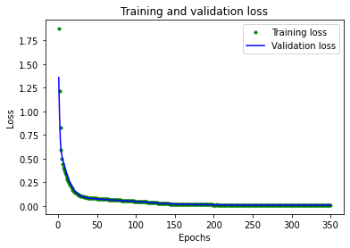
The loss rapidly decreased at the beginning before flattening out at the end. To make flatter part more readable let’s skip first 50 epochs:

1
2
3
4
5
6
7
8
9
SKIP = 50

plt.plot(epochs[SKIP:], loss[SKIP:],  'g.', label='Training loss')
plt.plot(epochs[SKIP:], validation_loss[SKIP:],  'b.', label='Validation loss')
plt.title('Training and validation loss')
plt.xlabel('Epochs')
plt.ylabel('Loss')
plt.legend()
plt.show()

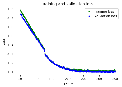
From the plot, we can see that loss continues to reduce until around 250 epochs, at which point it is mostly stable.

We can also see that the lowest loss value is around 0.0105. This means that our network’s predictions are off by an average of ~1%. Which is really good.

Let’s plot the mean absolute error, which is another way of measuring how far the network’s predictions are from the actual numbers:

1
2
3
4
5
6
7
8
9
10
mae = training_info.history['mae']
validation_mae = training_info.history['val_mae']

plt.plot(epochs[SKIP:], mae[SKIP:],  'g.', label='Training MAE')
plt.plot(epochs[SKIP:], validation_mae[SKIP:],  'b.', label='Validation MAE')
plt.title('Training and validation mean absolute error')
plt.xlabel('Epochs')
plt.ylabel('MAE')
plt.legend()
plt.show()

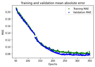
We can see that metrics are better for validation than training and that means the network is not overfitting. Our network seems to be performing well! To confirm, let’s check its predictions against the Test dataset we set aside earlier:

1
2
3
4
5
6
7
8
9
loss = model.evaluate(x_test, y_test)
predictions = model.predict(x_test)

plt.clf()
plt.title('Comparison of predictions and actual values')
plt.plot(x_test, y_test,  'b.', label='Actual')
plt.plot(x_test, predictions,  'r.', label='Predicted')
plt.legend()
plt.show()

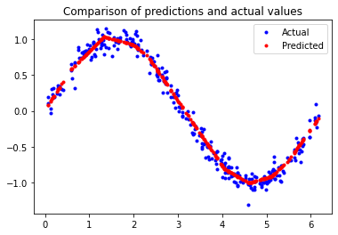
Looks really great! The model isn’t perfect; its predictions don’t form a smooth sine curve. If we wanted to go further, we could try further increasing the capacity of the model.

However, an important part of machine learning is knowing when to quit, and this model is good enough for our use case - which is to show a sine wave pattern on an LED and an LCD.

Generate a TensorFlow Lite Model

We now have an acceptably accurate model. We’ll use the TensorFlow Lite Converter to convert the model into a special, space-efficient format for use on memory-constrained devices.

1
2
3
4
converter = tf.lite.TFLiteConverter.from_keras_model(model)

converter.optimizations = [tf.lite.Optimize.DEFAULT]
tflite_model = converter.convert()

One of the optimization for hardware is quantization. In simple terms, fractional number (float, double) operations are expensive in microcontrollers. Input, output, weights, and biases are all float numbers. You might think converting these values into integer will reduce the model accuracy but in reality, most of the time, it is negligible. Of course, it will widely vary depending on the applications. But for our case, it is fine.

The tf.lite.Optimize.DEFAULT option will do its best to improve size and latency. This option will only quantize just the weights and not input and output. In my case, the output shows the file size is 2532 bytes (~2.5KB). Noice!

Let’s save the model:

1
open("sinewave_model.tflite",  "wb").write(tflite_model)

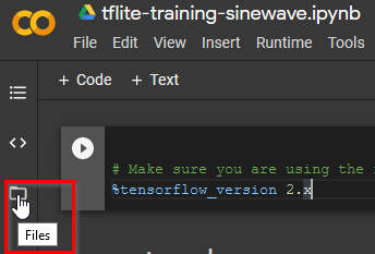
Now if you click the Files it will show you the folder structure.

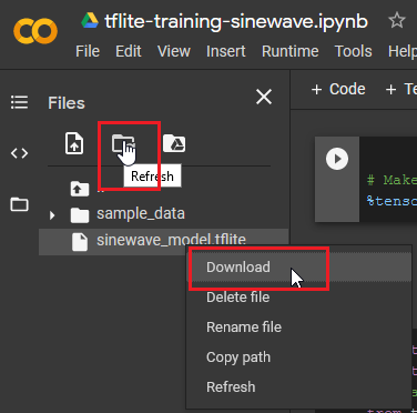
If the file doesn’t show up, click refresh. Right-click on the file, download and save it on your drive.

We actually don’t need this file. Unless you want to see the flow diagram of your model. Netron is a visualizer for neural network, deep learning, and machine learning models. Check their repo for more info.

Generate C files

Let’s generate the C source and header file of this model for the STM32 microcontroller. TF Lite has a Python method to convert the TF Lite model into C source and header files.

1
2
3
4
5
6
7
8
9
from tensorflow.lite.python.util import convert_bytes_to_c_source

source_text, header_text = convert_bytes_to_c_source(tflite_model,  "sine_model")

with  open('sine_model.h',  'w')  as  file:
    file.write(header_text)

with  open('sine_model.cc',  'w')  as  file:
    file.write(source_text)

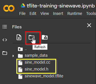
This will generate the C header and source file for you to use in your microcontroller. Download the files.

In the next part, I will show how to use these files on STM32Cube IDE.

Part-1: Introduction

Part-3: Running TFLite model on STM32